Analysis

Set Up

library(tidyverse)

── Attaching core tidyverse packages ──────────────────────── tidyverse 2.0.0 ──
✔ dplyr     1.1.4     ✔ readr     2.1.5
✔ forcats   1.0.0     ✔ stringr   1.5.1
✔ ggplot2   3.5.1     ✔ tibble    3.2.1
✔ lubridate 1.9.4     ✔ tidyr     1.3.1
✔ purrr     1.0.2     
── Conflicts ────────────────────────────────────────── tidyverse_conflicts() ──
✖ dplyr::filter() masks stats::filter()
✖ dplyr::lag()    masks stats::lag()
ℹ Use the conflicted package (<http://conflicted.r-lib.org/>) to force all conflicts to become errors

library(ggplot2)
load("data/df_clean.RData") # Load pre-cleaned data
load("data/gdp_long.RData")

Q1: Who Dominates

What are the top 10 medal-winning countries from 2020 to 2024?

# Create gradient color palette
color_paris <- colorRampPalette(c("#D8BFD8","#D796D5","#A89CDD","#9D9CC9"))(10) 

df1 <- df_clean2 |>
  filter(medal != "No medal",
         year >= 2000) |>
  group_by(country) |>
  summarise(num_of_medals = n()) |>
  arrange(-num_of_medals) |>
  head(10) |>
  mutate(country = fct_reorder(country, num_of_medals)) |>
  ggplot(aes(x = country,
             y = num_of_medals,
             fill = country)) +
  geom_col(width = 0.88) +
  geom_text(aes(label = num_of_medals), 
            hjust = -0.12, 
            size = 3,
            color = "brown",
            fontface = "bold") +
  geom_text(aes(label = country), 
            hjust = 1.1, 
            size = 3.5,
            color = "white",
            fontface = "bold") +
  coord_flip() +
  labs(x= "Country",
       y = "Total Medals",
       title = "Top 10 Medal-Winning Countries at the Olympics (2000–2024)",
       caption = "Source: Kaggle | Author: Huang Shixian") +
  scale_fill_manual(values = color_paris) +
  theme_light() +
  theme(panel.grid = element_blank(), 
        axis.text.y = element_blank(),
        axis.ticks.y = element_blank(),
        legend.position = "none",
        plot.title = element_text(face = "bold",
                                  size = 13,
                                  hjust = 0.5,
                                  margin = margin(b = 10)),
        axis.title.x = element_text(face = "bold",
                                    size = 12,
                                    color = "#3C2F60",
                                    margin = margin(t = 10)),
        axis.title.y = element_text(face = "bold",
                                    size = 12,
                                    color = "#3C2F60",
                                    margin = margin(r = 10)),
        plot.caption = element_text(margin = margin(t = 10)))
print(df1)

ggsave("q1.png", df1, width = 7, height = 4.2, dpi = 300)

Q2: How Gender Inclusion Develops

1) How has female participation in the Olympics grown over time?

df2 <- df_clean2 |>
  distinct(year, city, name, sex) |> # Remove duplicate athletes       
  group_by(year) |>                          
  summarise(total = n(),
            female = sum(sex == "F"), 
            city = first(city),
            percentage = female / total * 100,       
            .groups = "drop") |>
  mutate(olympics = paste(year, city),
         percentage2 = sprintf("%.1f%%", percentage)) |>
  ggplot(aes(x = olympics, 
             y = percentage,
             fill = year)) +
  scale_fill_gradientn(colors = c("#D3DFED", "#9BB5D4", "#6C8EBF", "#2F446D"),  
                      guide = "none") + 
  geom_col(width = 0.9) +
  geom_text(aes(label = percentage2),                      
            angle = 90,
            hjust = -0.1,
            vjust = 0.5,
            size = 2.8) +
  scale_y_continuous(limits = c(0, 55),
                     expand = c(0, 0),
                     name = "Percentage of Female Athletes") +
  scale_x_discrete(name = NULL) +             
  labs(title = "Growth of Female Participation in Summer Olympics Over Time",
       subtitle = "Note: The 1916, 1940, and 1944 Olympics were canceled due to World Wars I & II",
       caption = "Source: Kaggle | Author: Huang Shixian") +
  theme_minimal() +
  theme(axis.text.x = element_text(angle = 90, 
                               vjust = 0.5, 
                               size = 8, 
                               face = "bold"),
        panel.grid.major.x = element_blank(),
        plot.title = element_text(face = "bold", 
                              size = 14, 
                              hjust = 0.5,
                              margin = margin(b = 8)),
        plot.subtitle = element_text(size = 9, 
                                 color = "gray30",
                                 hjust = 0.5,
                                 margin = margin(b = 15)),
        plot.caption = element_text(margin = margin(t = 10)),
        axis.title.y = element_text(face = "bold"))
print(df2)

ggsave("q2.png", df2, width = 8, height = 5, dpi = 300)

2) How does the introduction year of female events vary across different Olympic sports?

df_introduction <- df_clean2 |>
  distinct(sport, year, name, sex) |>
  group_by(sport) |>
  summarise(introduction_year = ifelse(all(sex != "F"), NA, 
                                       min(year[sex == "F"]))) |>
  arrange(introduction_year) |>
  print()

# A tibble: 76 × 2
   sport          introduction_year
   <chr>                      <dbl>
 1 Croquet                     1900
 2 Equestrianism               1900
 3 Golf                        1900
 4 Sailing                     1900
 5 Tennis                      1900
 6 Archery                     1904
 7 Figure Skating              1908
 8 Motorboating                1908
 9 Diving                      1912
10 Swimming                    1912
# ℹ 66 more rows

# Check the the introduction year of Big Three
big_three <- df_introduction |> 
  filter(sport %in% c("Basketball","Volleyball","Football")) |>
  print()

# A tibble: 3 × 2
  sport      introduction_year
  <chr>                  <dbl>
1 Volleyball              1964
2 Basketball              1976
3 Football                1996

df_cumulative <- df_introduction |>
  count(year = introduction_year, 
        name = "female_sports") |>
  mutate(cumulative = cumsum(female_sports),
         total = n_distinct(df_clean2$sport),
         percentage = round(cumulative / total * 100, 1)) |>
  select(introduction_year = year, 
         female_sports = cumulative,
         percentage = percentage) |>
  print()

# A tibble: 24 × 3
   introduction_year female_sports percentage
               <dbl>         <int>      <dbl>
 1              1900             5        6.6
 2              1904             6        7.9
 3              1908             8       10.5
 4              1912            10       13.2
 5              1920            11       14.5
 6              1924            12       15.8
 7              1928            14       18.4
 8              1936            15       19.7
 9              1948            16       21.1
10              1964            17       22.4
# ℹ 14 more rows

Q3: How GDP Affects Medals

In Paris 2024, is there a measurable relationship between a country’s GDP and its Olympic performance?

df_performance <- df_clean2 |>
  filter(medal != "No medal",
         year == 2024) |>
  distinct(event, medal,country) |> 
  group_by(country) |>
  summarise(gold = sum(medal== "Gold"),
            silver = sum(medal == "Silver"), 
            bronze = sum(medal == "Bronze"),
            performance = gold*3 + silver*2 + bronze*1, # Weighted performance score  
            .groups = "drop") |>
  arrange(-performance) |>
  head(40) |>
  print()

# A tibble: 40 × 5
   country        gold silver bronze performance
   <chr>         <int>  <int>  <int>       <dbl>
 1 United States    37     42     39         234
 2 China            38     26     24         190
 3 Great Britain    13     22     28         111
 4 Australia        18     18     16         106
 5 France           13     22     22         105
 6 Japan            20     12     13          97
 7 Italy            12     11     13          71
 8 Netherlands      14      7     12          68
 9 Korea            13      9     10          67
10 Germany          11     10      8          61
# ℹ 30 more rows

df_gdp <- gdp_long |>
  filter(year >= 2020) |>
  group_by(country) |>
  summarise(avg_gdp = mean(gdp)) |>
  arrange(-avg_gdp) |>
  head(40) |>
  print()

# A tibble: 40 × 2
   country            avg_gdp
   <chr>                <dbl>
 1 United States      2.47e13
 2 China              1.70e13
 3 Japan              4.64e12
 4 Germany            4.24e12
 5 India              3.19e12
 6 Great Britain      3.08e12
 7 France             2.87e12
 8 Italy              2.12e12
 9 Canada             1.99e12
10 Russian Federation 1.91e12
# ℹ 30 more rows

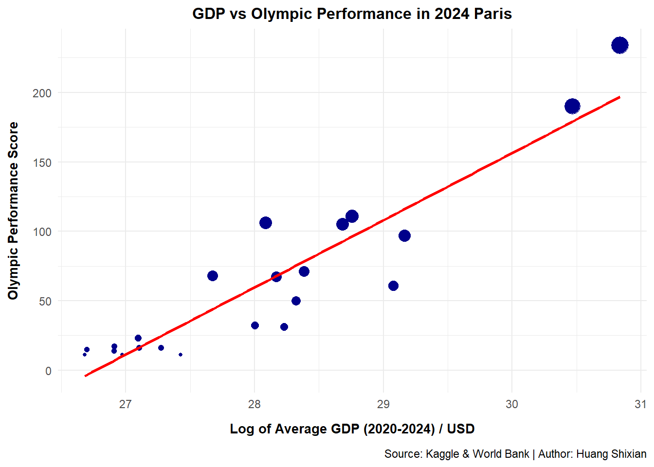
df3 <- df_performance |>
  inner_join(df_gdp, by = "country") # Merge two datasets

# Scatter plot with regression line
ggplot(df3, aes(x = log(avg_gdp), y = performance)) + # Logarithmic transformation
  geom_point(aes(size = performance), 
             color = "darkblue") +
  geom_smooth(method = "lm", 
              se = FALSE, 
              color = "red") +
  labs(x = "Log of Average GDP (2020-2024) / USD",
       y = "Olympic Performance Score",
       title = "GDP vs Olympic Performance in 2024 Paris",
       caption = "Source: Kaggle & World Bank | Author: Huang Shixian") +
  theme_minimal() +
  theme(legend.position = "none",
        plot.title = element_text(face = "bold", 
                              size = 12, 
                              hjust = 0.5),
        axis.title.x = element_text(face = "bold",
                                    size = 10,
                                    margin = margin(t = 10)),
        axis.title.y = element_text(face = "bold",
                                    size = 10,
                                    margin = margin(r = 10)),
        plot.caption = element_text(margin = margin(t = 10)),)

`geom_smooth()` using formula = 'y ~ x'

ggsave("q3.png", width = 7, height = 4.5, dpi = 300)

`geom_smooth()` using formula = 'y ~ x'

# Calculate Pearson correlation
correlation <- cor(log(df3$avg_gdp), df3$performance)
print(paste("Correlation (log GDP vs performance):", round(correlation, 3)))

[1] "Correlation (log GDP vs performance): 0.921"

# Estimate linear regression model
model <- lm(performance ~ log(avg_gdp), data = df3)
summary(model)

Call:
lm(formula = performance ~ log(avg_gdp), data = df3)

Residuals:
    Min      1Q  Median      3Q     Max 
-50.692 -16.369   4.044  14.142  42.211 

Coefficients:
              Estimate Std. Error t value Pr(>|t|)    
(Intercept)  -1294.209    128.327  -10.09 2.74e-09 ***
log(avg_gdp)    48.352      4.573   10.57 1.23e-09 ***
---
Signif. codes:  0 '***' 0.001 '**' 0.01 '*' 0.05 '.' 0.1 ' ' 1

Residual standard error: 23.95 on 20 degrees of freedom
Multiple R-squared:  0.8483,    Adjusted R-squared:  0.8407 
F-statistic: 111.8 on 1 and 20 DF,  p-value: 1.227e-09

# Compute residuals to identify outliers
df3$residuals <- residuals(model)
outliers <- df3[order(-abs(df3$residuals)), ] |> 
  head(5) |> 
  select(country, avg_gdp, performance, residuals) |>
  print()

# A tibble: 5 × 4
  country       avg_gdp performance residuals
  <chr>           <dbl>       <dbl>     <dbl>
1 Germany       4.24e12          61     -50.7
2 Australia     1.58e12         106      42.2
3 Brazil        1.82e12          31     -39.7
4 United States 2.47e13         234      37.2
5 Spain         1.45e12          32     -27.9

Case Study: Jamaica

# GDP analysis
jamaica_gdp <- gdp_long |>
  filter(country == "Jamaica", 
         year >= 2020) |>
  summarise(avg_gdp = mean(gdp, na.rm = TRUE)) |>
  print()

# A tibble: 1 × 1
       avg_gdp
         <dbl>
1 16247781016.

# Medal count
jamaica_medals <- df_clean2 |>
  filter(country == "Jamaica",
         year >= 2000,
         medal != "No medal") |>
  summarise(total_medals = n()) |>
  print()

# A tibble: 1 × 1
  total_medals
         <int>
1          132

# Sport distribution
jamaica_sport <- df_clean2 |>
  filter(country == "Jamaica",
         year >= 2000,
         medal != "No medal") |>
  group_by(sport) |>
  summarise(medals = n()) |>
  mutate(percentage = medals / sum(medals) * 100) |>
  arrange(-percentage) |>
  print()

# A tibble: 1 × 3
  sport     medals percentage
  <chr>      <int>      <dbl>
1 Athletics    132        100